Vizgen Mouse Brain
Note
Slide 1 Replicate 1
Introduction
This tutorial was written using Giotto version 2.0.0.9045. Check the version you are using to get the same results. If you do not have Giotto installed, you can do so by running the following code.
remotes::install_github("RubD/Giotto@suite")
Now, load the library and define the project path.
library(Giotto)

# 1. set working directory
results_folder = '/path/to/directory/'

# 2. set giotto python path
# set python path to your preferred python version path
# set python path to NULL if you want to automatically install (only the 1st
# time) and use the giotto miniconda environment
python_path = NULL
if(is.null(python_path)) {
installGiottoEnvironment()
}
Dataset Explanation
This tutorial uses the neuroscience showcase data provided by the Vizgen company. It captures transcripts at subcellular resolution and outputs:
List of all detected transcripts and their spatial locations in three dimensions (CSV)
The DAPI and Poly T mosaic images (TIFF)
Output from the cell segmentation analysis: the transcripts per cell matrix (CSV), the cell metadata (CSV) and the cell boundaries (HDF5)
The company mapped the mouse brain in 9 full slices across 3 positions. However, this tutorial only uses the first replicate from the first slide.
Giotto global instructions and preparations
Define the instructions to save the plots.
# by directly saving plots, but not rendering them you will save a lot of time
instrs = createGiottoInstructions(save_dir = results_folder,
                save_plot = TRUE,
                show_plot = FALSE,
                return_plot = FALSE)
Create Giotto object and process data
To create the Giotto object, you first need to read the cell by gene expression matrix and the metadata information. Since Giotto receives the expression with genes as rows and cells as columns, you need to transpose the expression matrix to create the object.
The Vizgen data comes with information about the field of view (FOV) and the volume of the cell. This metadata information can be added to the object.
# provide path to cell by gene matrix
expr_path = '/path/to/datasets_mouse_brain_map_BrainReceptorShowcase_Slice1_Replicate1_cell_by_gene_S1R1.csv'
# provide path to metadata
spat_path = '/path/to/datasets_mouse_brain_map_BrainReceptorShowcase_Slice1_Replicate1_cell_metadata_S1R1.csv'

# read expression matrix and metadata
expr_matrix = readExprMatrix(expr_path)
spat_dt = data.table::fread(spat_path)

# create giotto object
vizgen <- createGiottoObject(expression = Giotto:::t_flex(expr_matrix),
                spatial_locs = spat_dt[,.(center_x, center_y, V1)],
                instructions = instrs)
# add metadata of fov and volume
vizgen <- addCellMetadata(vizgen, new_metadata = spat_dt[,.(fov, volume)])
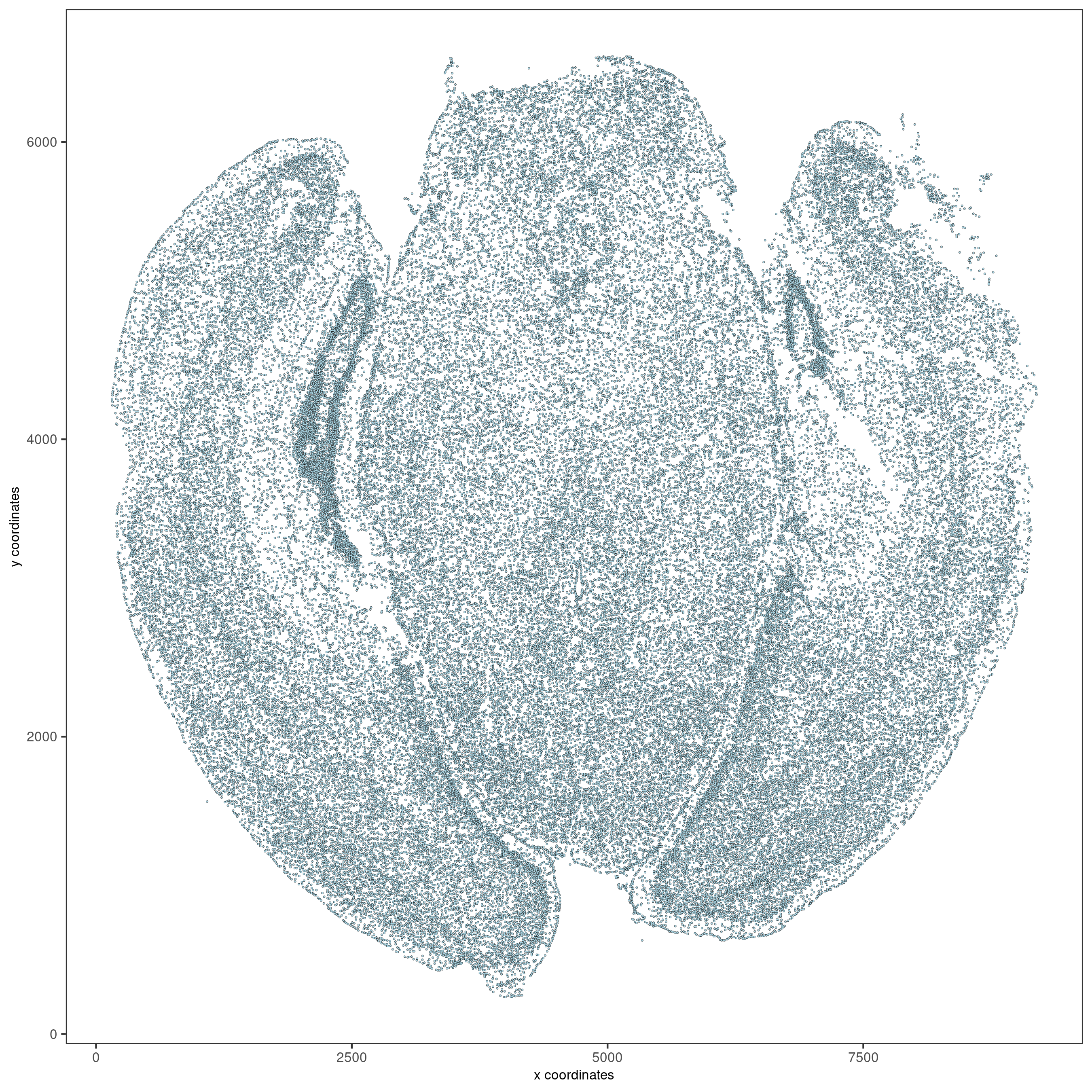
Visualize cells in space.
spatPlot2D(vizgen, point_size = 0.5, show_plot = F, return_plot = F,
       save_plot = T, save_param = list(show_saved_plot = TRUE))
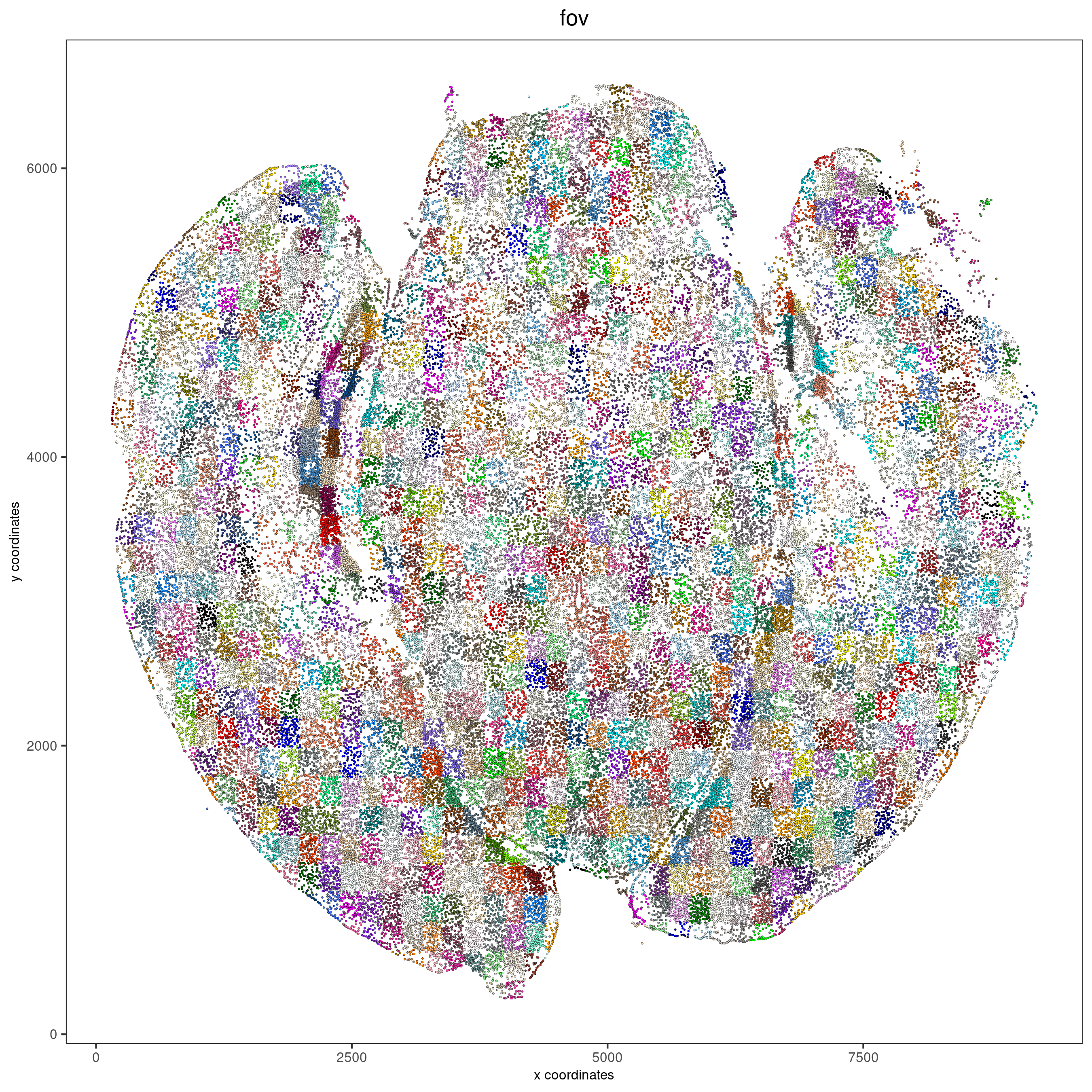
Visualize cells by FOV.
spatPlot2D(vizgen, point_size = 0.5, cell_color = 'fov', show_legend = F,
       show_plot = F, return_plot = F, save_plot = T,
       save_param = list(show_saved_plot = TRUE))
Processing steps.
vizgen <- filterGiotto(gobject = vizgen,
           expression_threshold = 1,
           feat_det_in_min_cells = 100,
           min_det_feats_per_cell = 20)
vizgen <- normalizeGiotto(gobject = vizgen, scalefactor = 1000, verbose = T)
# add gene and cell statistics
vizgen <- addStatistics(gobject = vizgen)
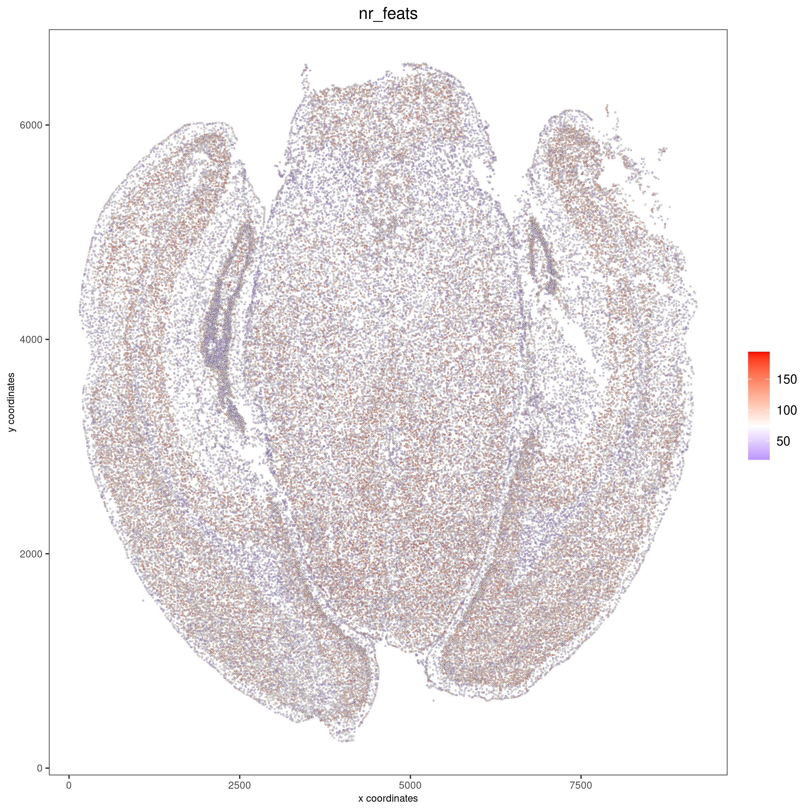
Visualize the number of features per cell.
spatPlot2D(gobject = vizgen_brain, show_image = F, point_alpha = 0.7,
       cell_color = 'nr_feats', color_as_factor = F, point_size = 0.5,
       save_param = list(show_saved_plot = TRUE))
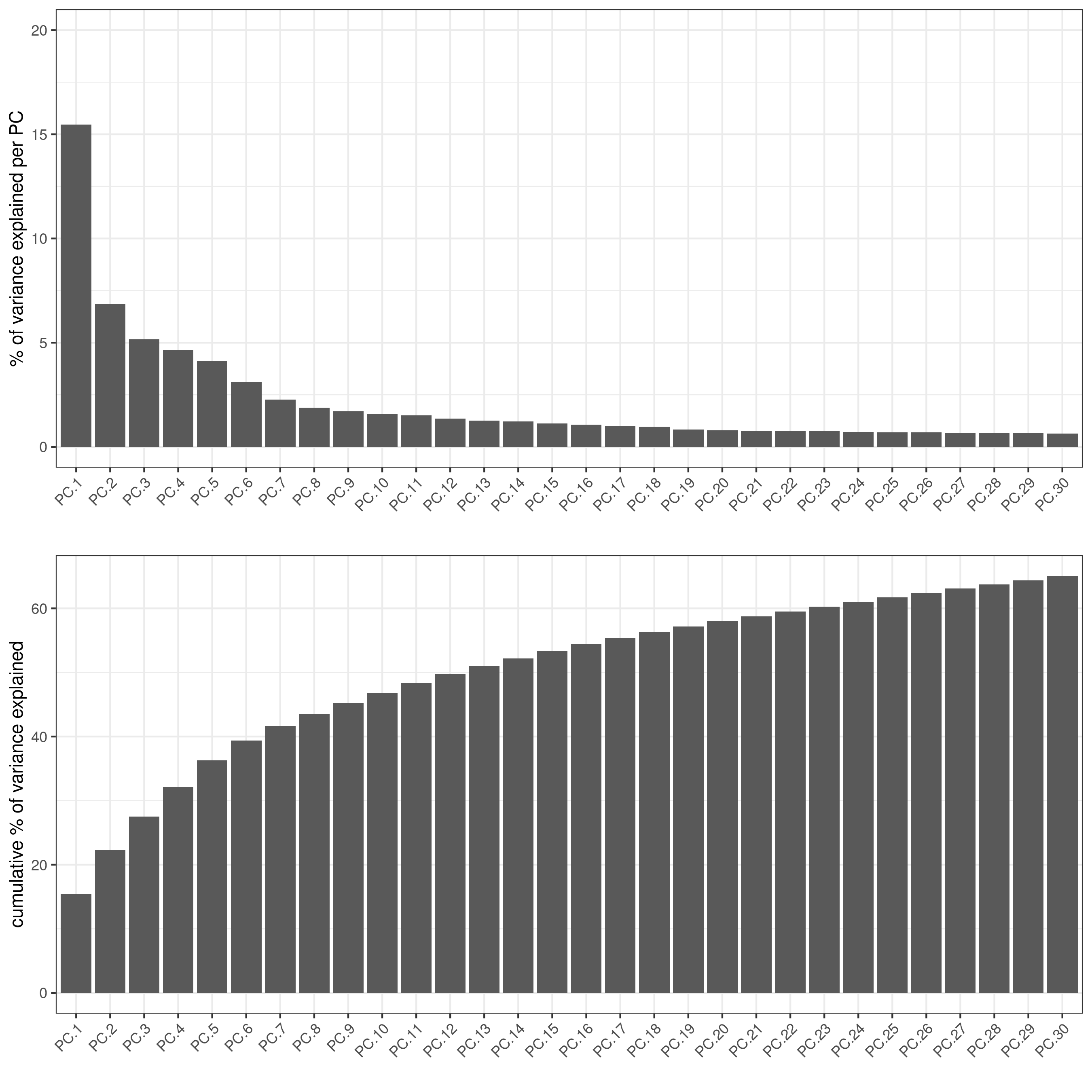
Dimension Reduction
Since no HVG selection was performed, Giotto will consider all genes. The first step is to calculate the principal components. .. code-block:
vizgen <- runPCA(gobject = vizgen, center = TRUE, scale_unit = TRUE)
# visualize variance explained per component
screePlot(vizgen, ncp = 30)
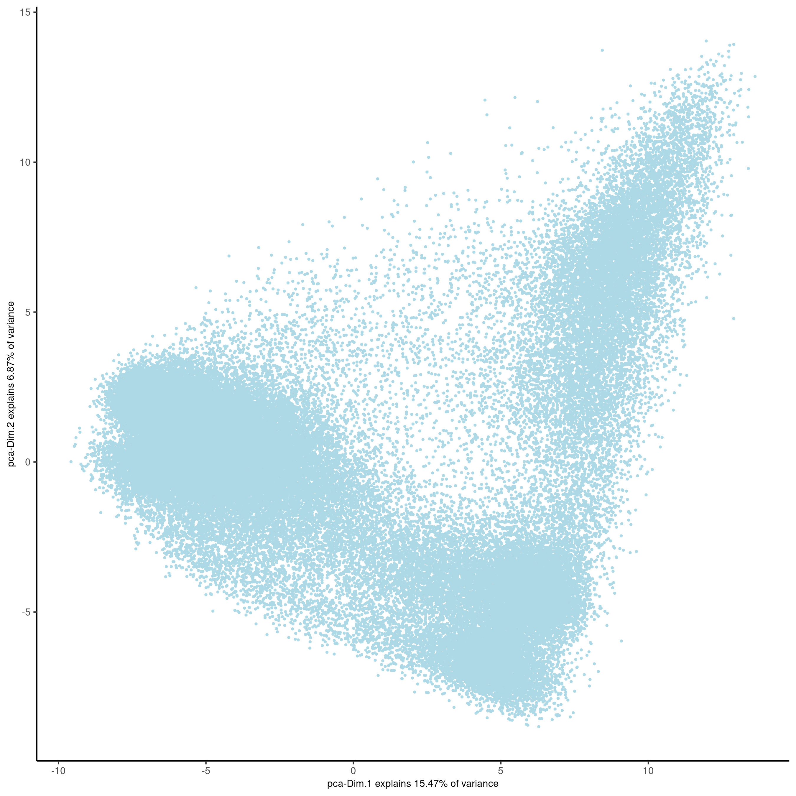
plotPCA(gobject = vizgen, point_size = 0.5, show_plot = F, return_plot = F,
    save_plot = T, save_param = list(show_saved_plot = TRUE))
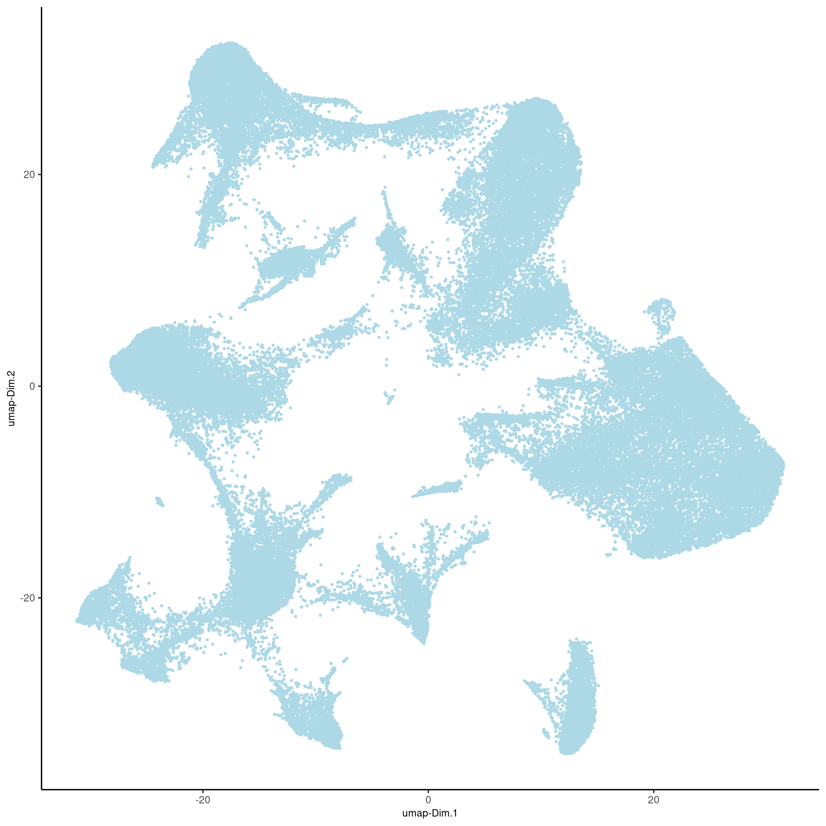
vizgen = runUMAP(vizgen, dimensions_to_use = 1:10)
 plotUMAP(gobject = vizgen, point_size = 0.5, show_plot = F, return_plot = F,
     save_plot = T, save_param = list(show_saved_plot = TRUE))
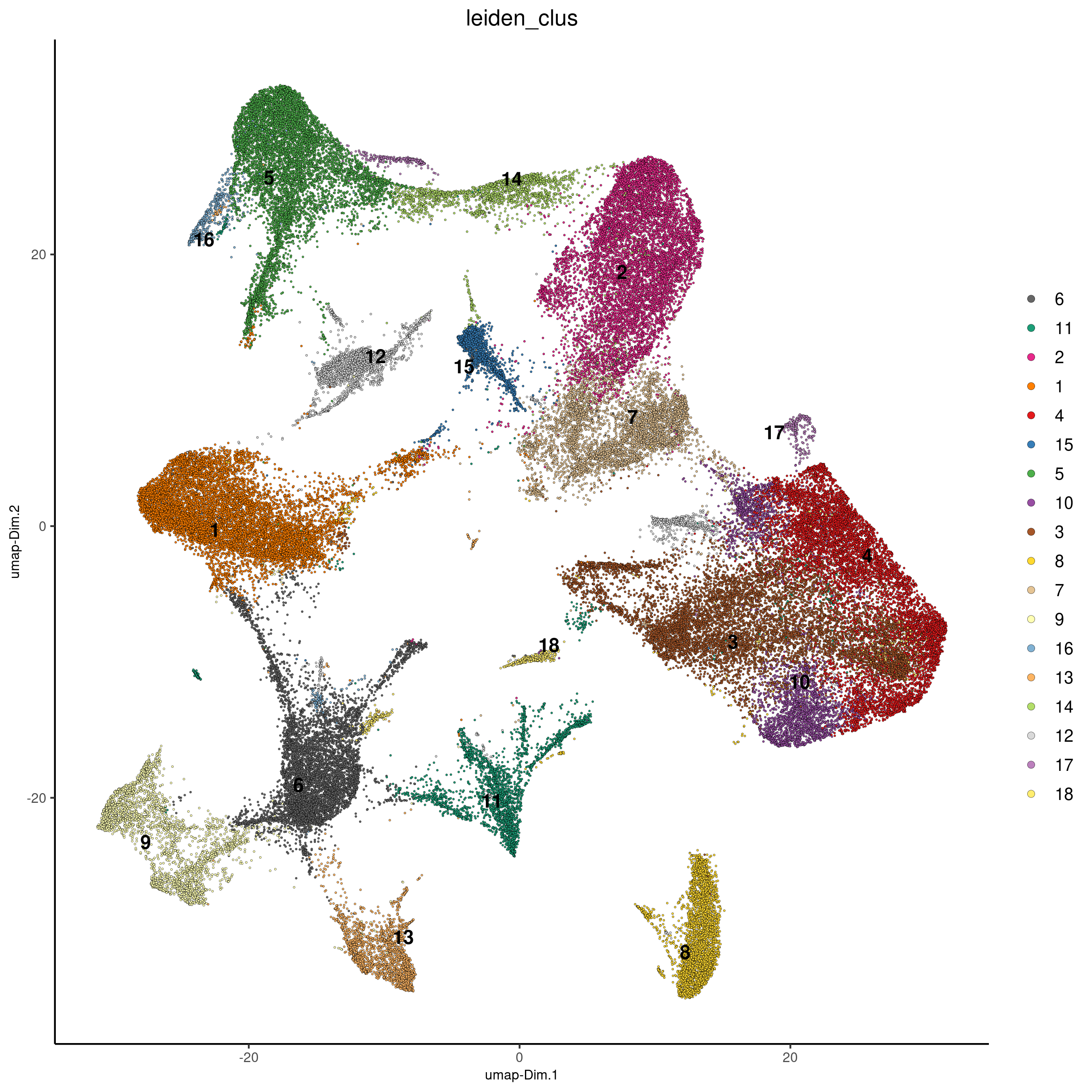
Cluster
Calculate nearest neighbor network and perform Leiden clustering.
vizgen <- createNearestNetwork(vizgen, dimensions_to_use = 1:10, k = 15)
vizgen <- doLeidenCluster(vizgen, resolution = 0.2, n_iterations = 100)
Visualize clusters in reduced dimension. The default cell color is ‘leiden_clus’.
plotUMAP(vizgen, cell_color = 'leiden_clus', point_size = 0.5, show_plot = F,
     return_plot = F, save_plot = T,
     save_param = list(show_saved_plot = TRUE))
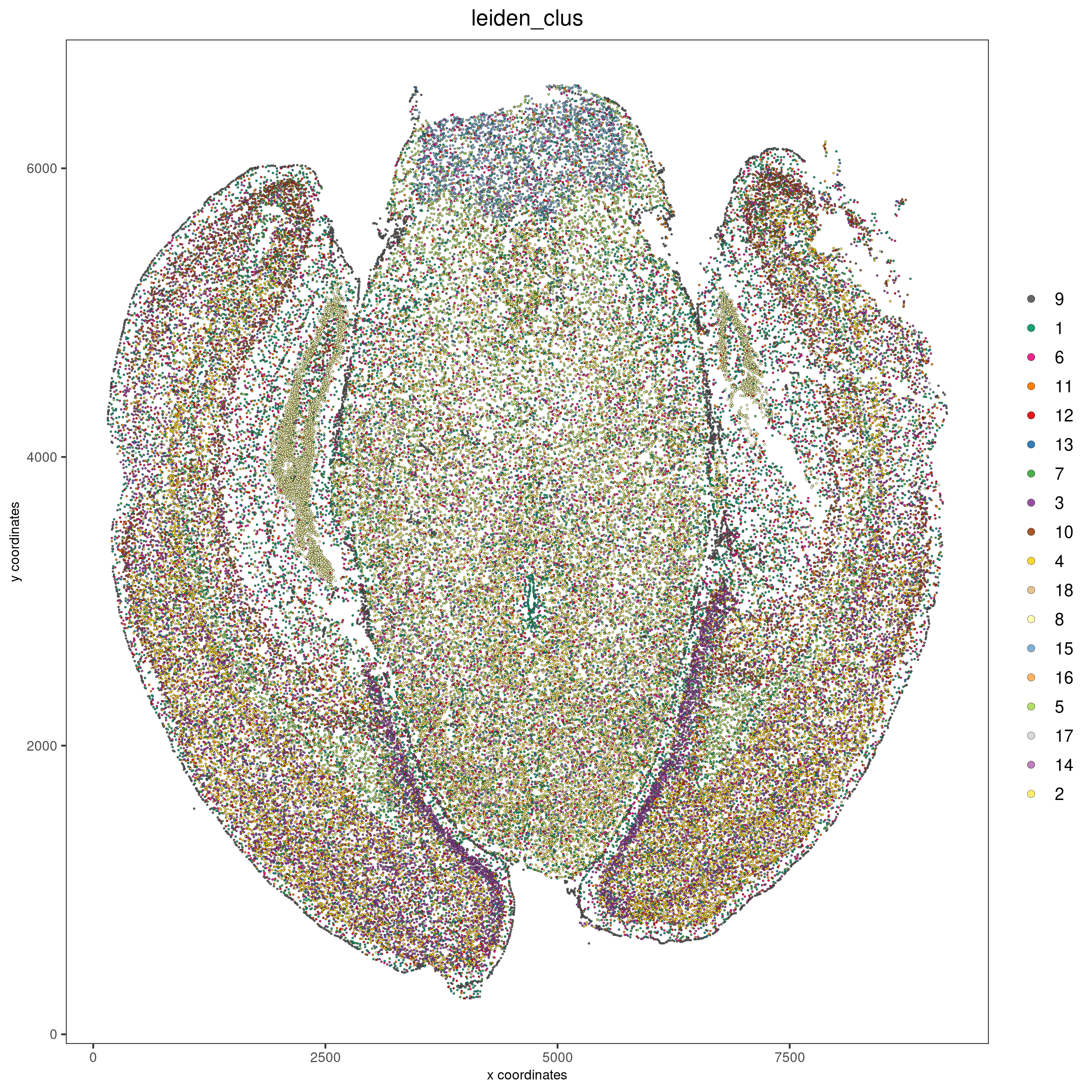
Visualize in spatial dimensions.
spatPlot2D(gobject = vizgen, cell_color = 'leiden_clus', point_size = 0.5,
       show_plot = F, return_plot = F, save_plot = T,
       save_param = list(show_saved_plot = TRUE))
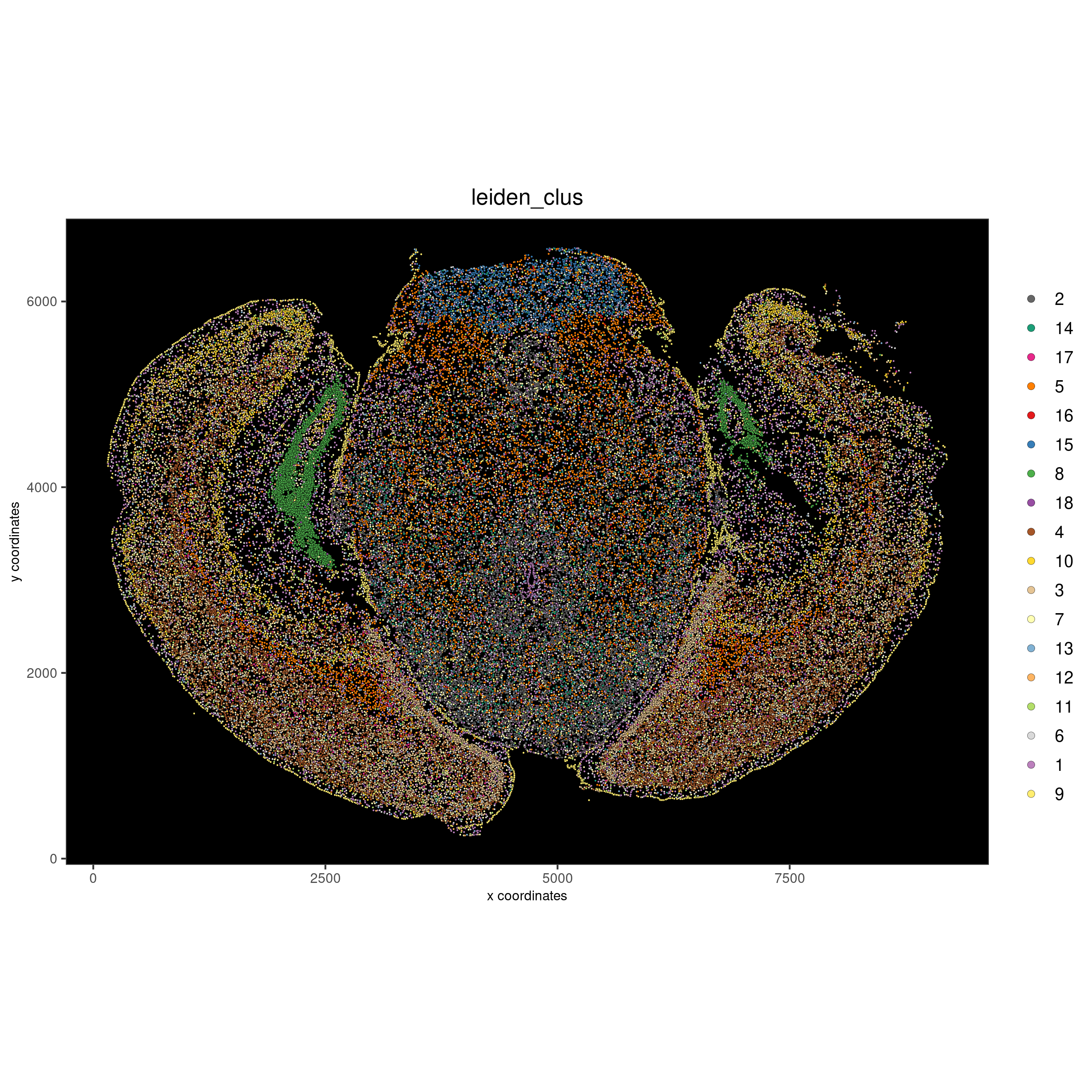
It is also possible to reverse the colors for the visualization.
# get colors
cell_metadata = pDataDT(vizgen)
leiden_names = unique(cell_metadata$leiden)
leiden_colors = Giotto::getDistinctColors(n = length(leiden_names))
names(leiden_colors) = leiden_names

# reverse colors
leiden_rev_colors = Giotto::getDistinctColors(n = length(leiden_names))
names(leiden_rev_colors) = rev(leiden_names)

# visualize with reversed colors
spatPlot2D(gobject = vizgen, cell_color = 'leiden_clus', point_size = 0.5,
    cell_color_code = leiden_rev_colors, coord_fix_ratio = TRUE,
    background_color = 'black', show_plot = F, return_plot = F,
    save_plot = T, save_param = list(show_saved_plot = TRUE))
Spatial expression patterns
The first step is to calculate the spatial network and then perform the binary spatial extraction of genes.
# create spatial network based on physical distance of cell centroids
vizgen = createSpatialNetwork(gobject = vizgen, minimum_k = 2,
maximum_distance_delaunay = 50)
# select features
feats = vizgen@feat_ID$rna
# perform Binary Spatial Extraction of genes
km_spatialgenes = binSpect(vizgen, subset_feats = feats)
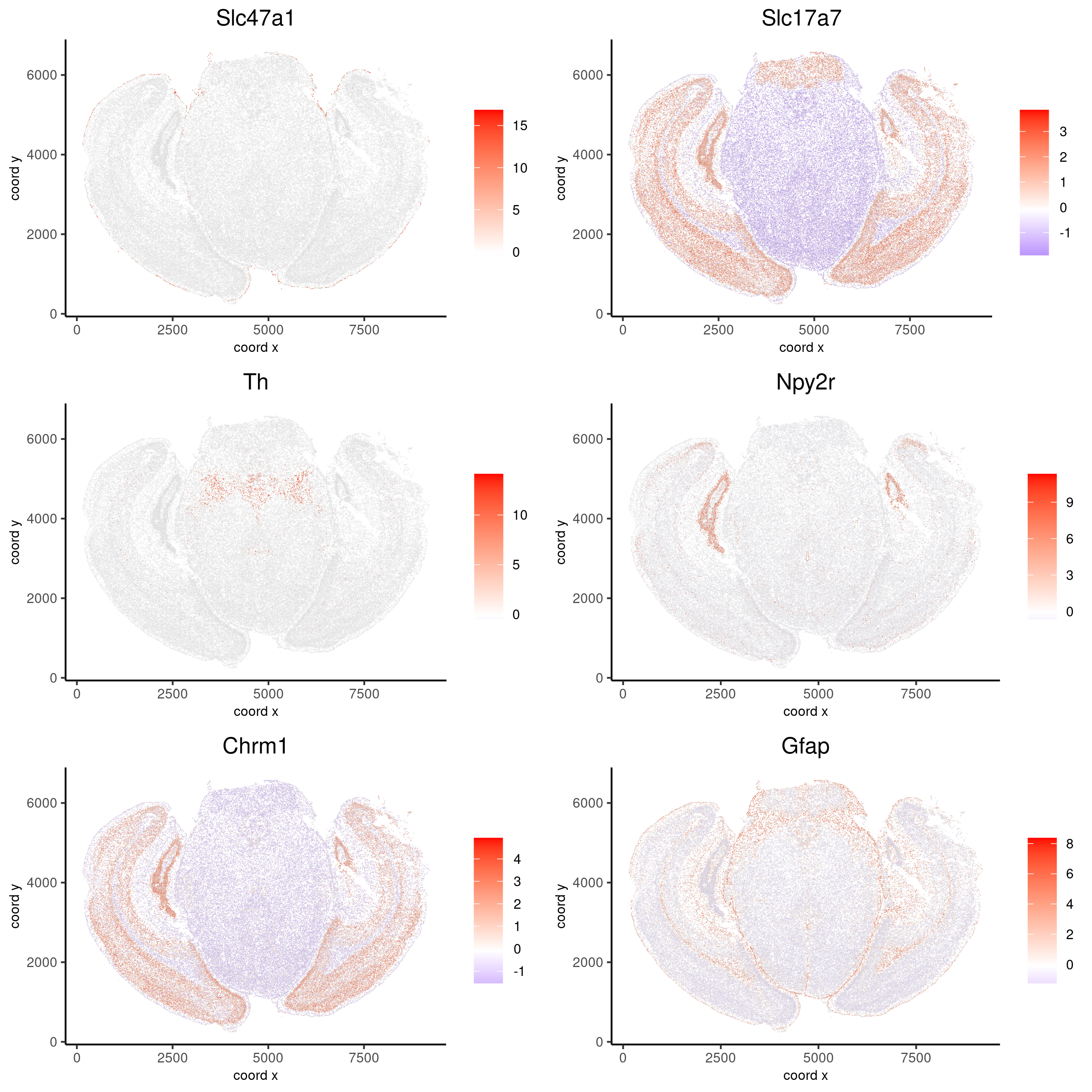
# visualize spatial expression of selected genes obtained from binSpect
spatFeatPlot2D(vizgen, expression_values = 'scaled',
feats = c('Slc47a1', 'Slc17a7', 'Th', 'Npy2r', 'Chrm1', 'Gfap'),
cell_color_gradient = c('blue', 'white', 'red'),
point_shape = 'border', point_border_stroke = 0.01,
show_network = F, network_color = 'lightgrey', point_size = 0.2,
cow_n_col = 2)
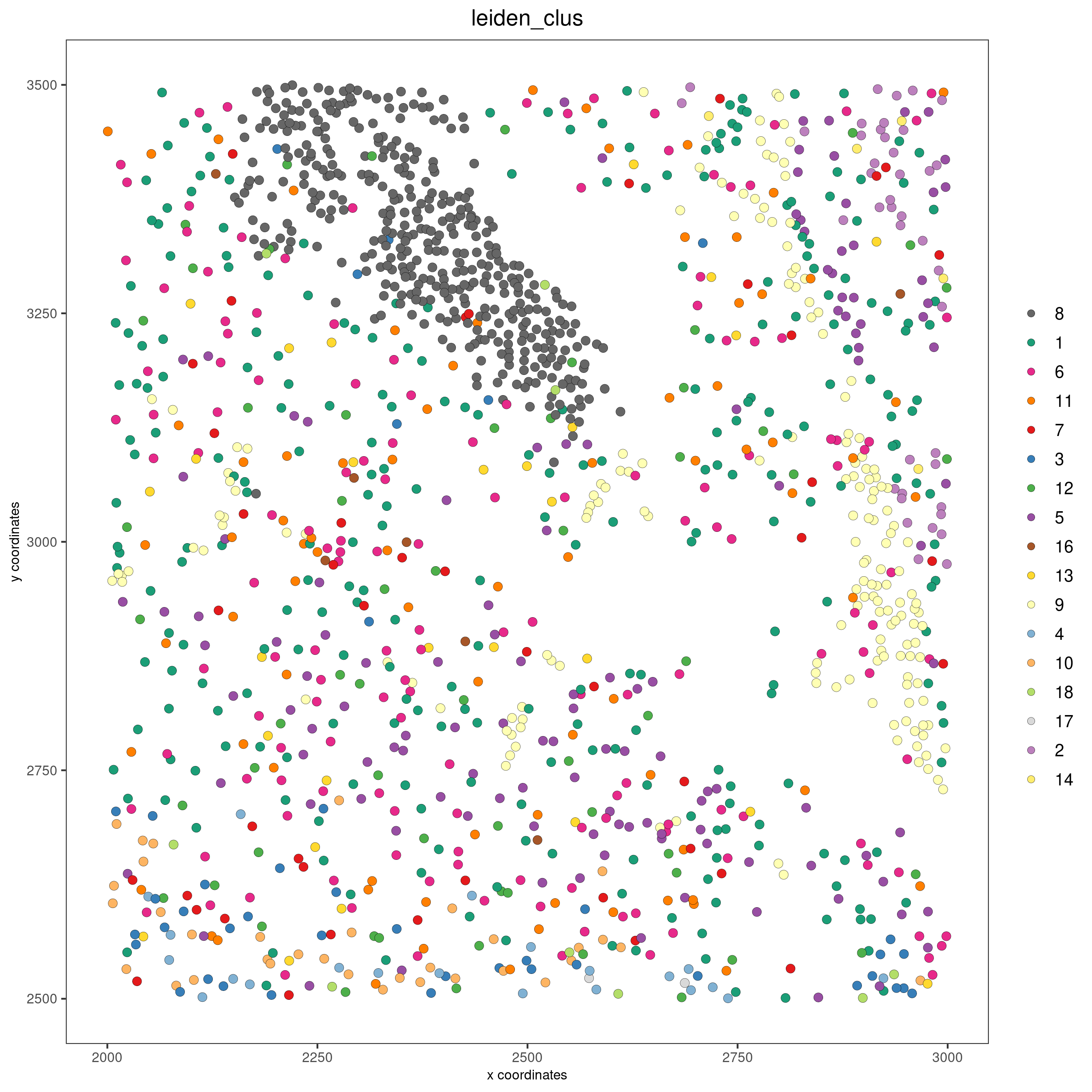
Subset Giotto and add cell boundary information
Giotto can be subset to analyze only a portion of the data.
vizgen_subset <- subsetGiottoLocs(gobject = vizgen,
                  x_min = 2000, x_max = 3000,
                  y_max = 3500, y_min = 2500)
The visualization functions can also be applied to the subset version.
spatPlot2D(gobject = vizgen_subset, cell_color = 'leiden_clus', point_size = 2.5,
    show_plot = F, return_plot = F, save_plot = T,
    save_param = list(show_saved_plot = TRUE))
Giotto can include the information about the polygons as provided by Vizgen. Since we are working with a subset of the data, it is necessary to read only the polygons that are present in the current FOVs.
# define path to cell boundaries folder
bound_path = '/path/to/cell_boundaries'
# read polygons and add them to Giotto
vizgen_subset = readPolygonFilesVizgen(gobject = vizgen_subset,
                    boundaries_path = bound_path,
                    polygon_feat_types = c(0,4,6))
Giotto can also include information about the transcripts.
# add transcript coordinates
tx_path = '/path/to/datasets_mouse_brain_map_BrainReceptorShowcase_Slice1_Replicate1_detected_transcripts_S1R1.csv'
tx_dt = data.table::fread(tx_path)
# select transcripts in FOVs
selected_fovs = unique(pDataDT(vizgen_subset)$fov)
tx_dt_selected = tx_dt[fov %in% selected_fovs]
# create Giotto points from transcripts
gpoints = createGiottoPoints(x = tx_dt_selected[,.(global_x,global_y, gene)])
# add points to Giotto
vizgen_subset = addGiottoPoints(gobject = vizgen_subset,
gpoints = list(gpoints))
# identify genes for visualization
gene_meta = fDataDT(vizgen_subset)
data.table::setorder(gene_meta, perc_cells)
gene_meta[perc_cells > 25 & perc_cells < 50]
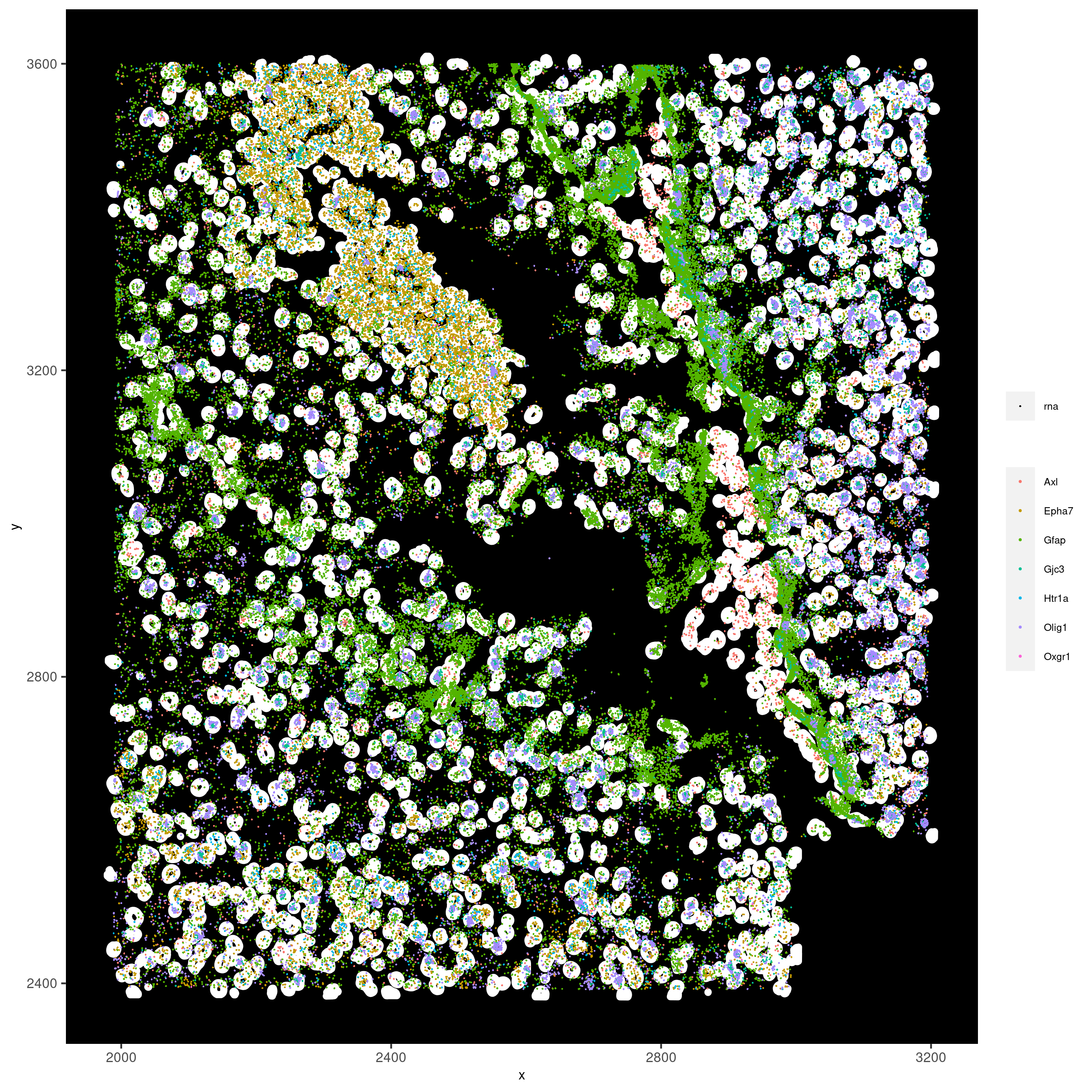
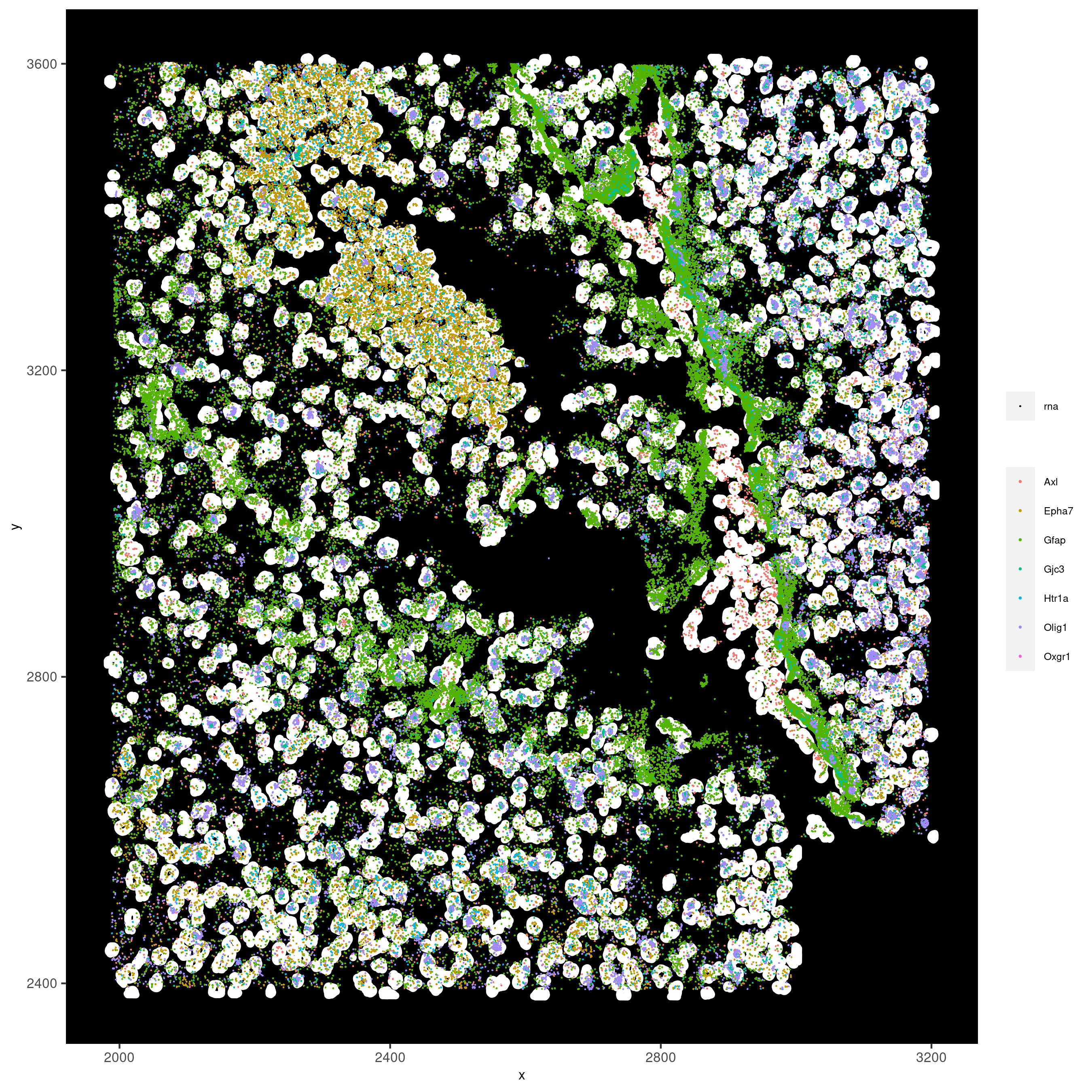
# visualize points from index z0
spatInSituPlotPoints(vizgen_subset,
feats = list('rna' = c("Oxgr1", "Htr1a", "Gjc3", "Axl",
'Gfap', "Olig1", "Epha7")),
polygon_feat_type = 'z0',
use_overlap = F,
point_size = 0.2,
show_polygon = TRUE,
polygon_color = 'white',
return_plot = FALSE,
save_plot = TRUE,
show_plot = FALSE,
save_param = list(show_saved_plot = TRUE))
# visualize points from index z6
spatInSituPlotPoints(vizgen_subset,
            feats = list('rna' = c("Oxgr1", "Htr1a", "Gjc3", "Axl",
                        'Gfap', "Olig1", "Epha7")),
            polygon_feat_type = 'z6',
            use_overlap = F,
            point_size = 0.2,
            show_polygon = TRUE,
            polygon_color = 'white',
            return_plot = FALSE,
            save_plot = TRUE,
            show_plot = FALSE,
            save_param = list(show_saved_plot = TRUE))