Integration of Single Cell Data

Set up Giotto Environment

library(Giotto)

# 1. set working directory
results_folder = 'path/to/result'

# 2. set giotto python path
# set python path to your preferred python version path
# set python path to conda env/bin/ directory if manually installed Giotto python dependencies by conda
# python_path = '/path_to_conda/.conda/envs/giotto/bin/python'
# set python path to NULL if you want to automatically install (only the 1st time) and use the giotto miniconda environment
python_path = NULL
if(is.null(python_path)) {
installGiottoEnvironment()
}

# 3. create giotto instructions
instrs = createGiottoInstructions(save_dir = results_folder,
                                save_plot = TRUE,
                                show_plot = FALSE,
                                python_path = python_path)

Dataset Explanation

This is a tutorial for Harmony integration of different single cell RNAseq datasets using two prostate cancer patient datasets. Ma et al. Processed 10X Single Cell RNAseq from two prostate cancer patients. The raw dataset can be found here

Part 1: Create Giotto object from 10X dataset and join

giotto_P1<-createGiottoObject(expression = get10Xmatrix("path/to/P1_result/outs/filtered_feature_bc_matrix",
                gene_column_index = 2, remove_zero_rows = TRUE),
                instructions = instrs)

giotto_P2<-createGiottoObject(expression = get10Xmatrix("path/to/P2_result/outs/filtered_feature_bc_matrix",
                            gene_column_index = 2, remove_zero_rows = TRUE),
                instructions = instrs)
giotto_SC_join = joinGiottoObjects(gobject_list = list(giotto_P1, giotto_P2),
                gobject_names = c('P1', 'P2'),
                join_method = "z_stack")

Part 2: Process Joined object

giotto_SC_join <- filterGiotto(gobject = giotto_SC_join,
expression_threshold = 1,
feat_det_in_min_cells = 50,
min_det_feats_per_cell = 500,
expression_values = c('raw'),
verbose = T)

## normalize
giotto_SC_join <- normalizeGiotto(gobject = giotto_SC_join, scalefactor = 6000)

## add gene & cell statistics
giotto_SC_join <- addStatistics(gobject = giotto_SC_join, expression_values = 'raw')

Part 3: Dimention reduction and clustering

## PCA ##
giotto_SC_join <- calculateHVF(gobject = giotto_SC_join)
giotto_SC_join <- runPCA(gobject = giotto_SC_join, center = TRUE, scale_unit = TRUE)
# Check screeplot to select number of PCs for clustering
# screePlot(giotto_SC_join, ncp = 30, save_param = list(save_name = '3_scree_plot'))

## WITHOUT INTEGRATION ##
# --------------------- #

## cluster and run UMAP ##
# sNN network (default)
showGiottoDimRed(giotto_SC_join)
giotto_SC_join <- createNearestNetwork(gobject = giotto_SC_join,
    dim_reduction_to_use = 'pca', dim_reduction_name = 'pca',
    dimensions_to_use = 1:10, k = 15)

# Leiden clustering
giotto_SC_join <- doLeidenCluster(gobject = giotto_SC_join, resolution = 0.2, n_iterations = 1000)

# UMAP
giotto_SC_join = runUMAP(giotto_SC_join)

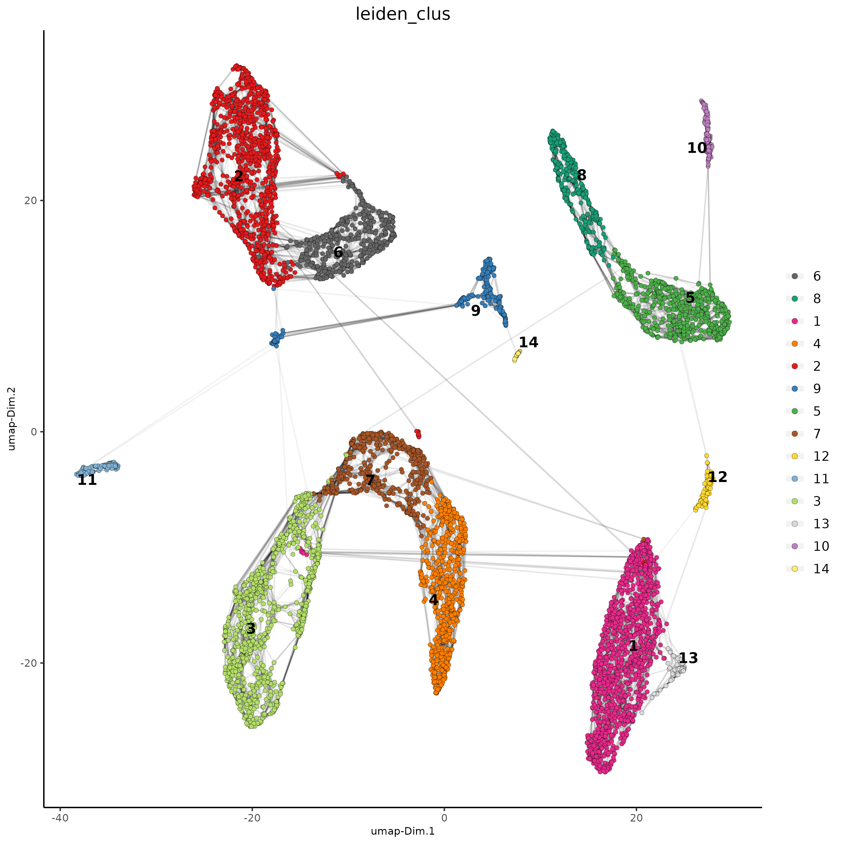
plotUMAP(gobject = giotto_SC_join,
    cell_color = 'leiden_clus', show_NN_network = T, point_size = 1.5,
    save_param = list(save_name = "4_cluster_without_integration"))

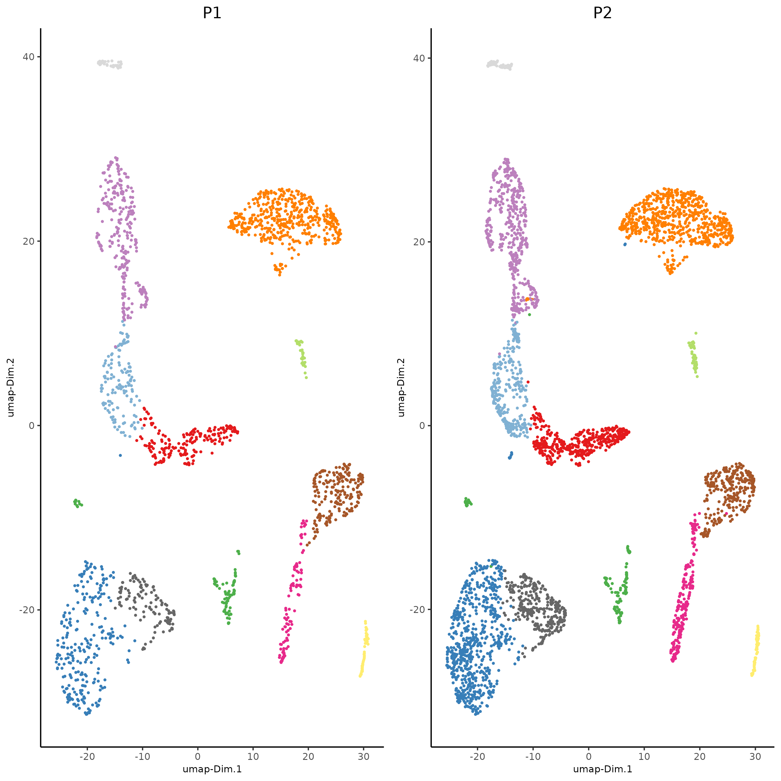
dimPlot2D(gobject = giotto_SC_join, dim_reduction_name = 'umap', point_shape = 'no_border',
cell_color = "leiden_clus", group_by = "list_ID", show_NN_network = F, point_size = 0.5,
show_center_label = F, show_legend =F,
save_param = list(save_name = "4_list_without_integration"))

Note

Harmony is a integration algorithm developed by Korsunsky, I. et al.. It was designed for integration of single cell data but also work well on spatial datasets.

## WITH INTEGRATION ##
# --------------------- #

## data integration, cluster and run UMAP ##

# harmony
#library(devtools)
#install_github("immunogenomics/harmony")
library(harmony)

#pDataDT(giotto_SC_join)
giotto_SC_join = runGiottoHarmony(giotto_SC_join, vars_use = 'list_ID', do_pca = F)


## sNN network (default)
#showGiottoDimRed(giotto_SC_join)
giotto_SC_join <- createNearestNetwork(gobject = giotto_SC_join,
    dim_reduction_to_use = 'harmony', dim_reduction_name = 'harmony', name = 'NN.harmony',
    dimensions_to_use = 1:10, k = 15)

## Leiden clustering
giotto_SC_join <- doLeidenCluster(gobject = giotto_SC_join,
    network_name = 'NN.harmony', resolution = 0.2, n_iterations = 1000, name = 'leiden_harmony')

# UMAP dimension reduction
#showGiottoDimRed(giotto_SC_join)
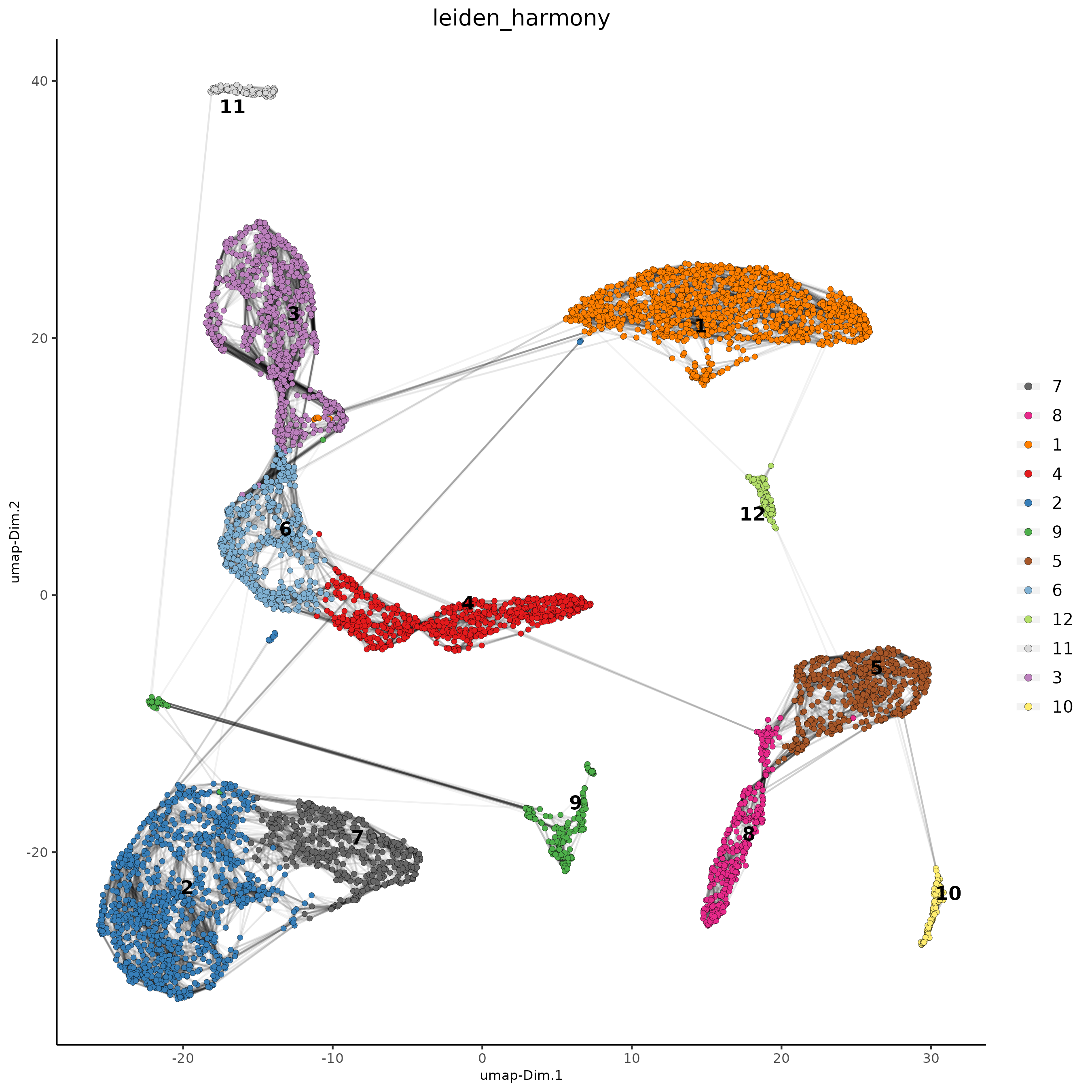
giotto_SC_join = runUMAP(giotto_SC_join, dim_reduction_name = 'harmony', dim_reduction_to_use = 'harmony', name = 'umap_harmony')
plotUMAP(gobject = giotto_SC_join,
    dim_reduction_name = 'umap_harmony',
    cell_color = 'leiden_harmony', show_NN_network = T, point_size = 1.5,
    save_param = list(save_name = "4_cluster_with_integration"))

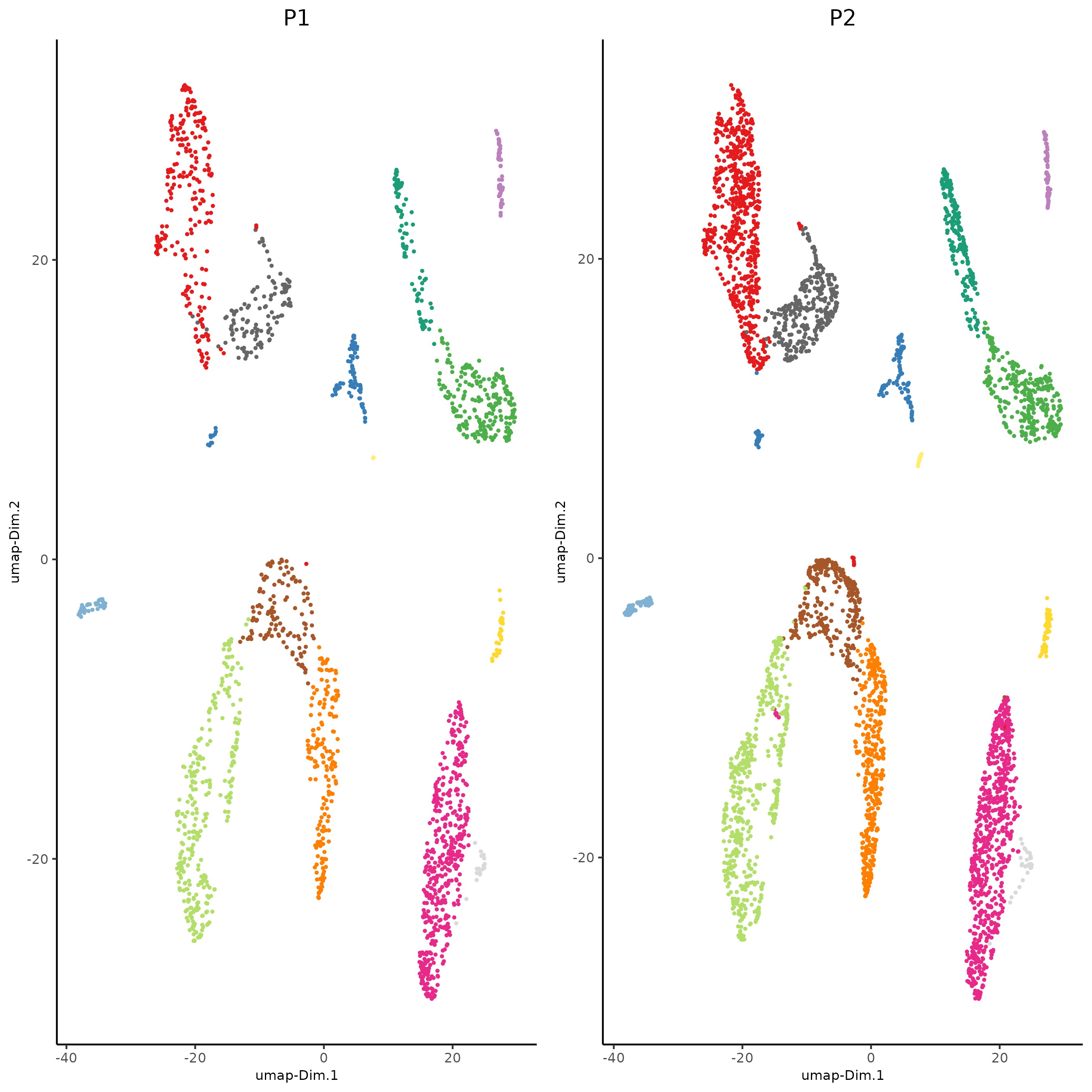
dimPlot2D(gobject = giotto_SC_join,     dim_reduction_name = 'umap_harmony', point_shape = 'no_border',
cell_color = "leiden_harmony", group_by = "list_ID", show_NN_network = F, point_size = 0.5,
show_center_label = F, show_legend =F , save_param = list(save_name = "4_list_with_integration"))